ANFIS and MLP solutions for the inverse kinematics of the 3R planar manipulator. N.B. There is NO going into depth on how ANFIS or MLP work. I am just an API WORKER in this post.
QUICK LINK: For the coursework report and codes, click JinhangZhu/ias-coursework.
- Some related examples
- Inverse Kinematics via Learning
- Data generation
- Implementations
- Evaluation
- Analysis of Results
- Conclusion
- References
Some related examples
Many approaches can solve the inverse kinematics problems of a robot manipulator. Traditional methods, including the closed-form solutions and numerical solutions (Craig, Prentice, and Hall 2005), can solve the IK problems either in a direct mathematical way or in an iterative manner. However, as the complexity of the robot manipulators increase, the non-linearity in the IK functions rises, and these traditional methods are proved to be time-consuming (Alavandar et al. 2008)(Koker et al. 2004). Meanwhile, the neural networks present higher capabilities of learning and nonlinear functions approximations. Therefore, machine learning-based methods are suitable for solving the inverse kinematics problems in complex robot manipulators (Alavandar et al. 2008). Fuzzy Inference Systems have more advantages in soft computing, which makes it suitable for the calculation for continuous trajectories of the robot end-effector. To automate the process of tuning membership functions of FIS, researchers proposed ANFIS, i.e. combination of neural networks and FIS.
Duka (2015) considered the inverse kinematics of a planar 3 degree of freedom (DOF) robot as a fitting problem. They simulated the IK problem via mapping the end-effector's (EE's) localisation to the joint angular space by the mean of ANFIS. One significant contribution is that they first applied EE pose in ANFIS model learning. The localisation vectors, with duplicates removed, were fed to three ANFIS networks and each of which has six membership functions (MFs). They predict the joint angles $\theta_1$, $\theta_2$ and $\theta_3$, respectively. However, the paper did not explain which number of MFs yields the best results even it declared 3, 5, 6 were tried in training. Also, the number of training samples (1000) and the number of epochs (200) were not proved by the paper to be the best choice so further exploration in the two configurations could be done.
Proposed by Alavandar et al. (2008), the ANFIS model has $49$ rules in total and the membership functions are Gaussian-type. The 2 DOF planar manipulator has link lengths: $l_1=10$, $l_2=7$ and angle limits: $\theta_1 , [0,\pi/2], \theta_2 , [0,\pi]$, showing that the geometrical configurations are as same as those of the MATLAB examples. Two ANFIS models are respectively for theta1 and theta2, learning from the data of mapped vectors of locations and angles. Also, the paper studied the IK problem of a $3$ DOF planar redundant manipulator. The ANFIS network takes coordinates and angles as the training data with Gaussian membership function with hybrid learning. However, they did not demonstrate the information about how the learning process is implemented.
Duka (2014) considered a hypothetical three-link planar manipulator with rotational joints. The inverse kinematics problem is to make the robotic arm track a circular trajectory in its workspace. Before building the feed-forward network, they generate $1000$ uniformly randomised sets of joint angles and apply forward kinematics to calculate the corresponding Cartesian coordinates and the orientations. Since the $3$ DOF manipulator can hold multiple IK solutions to the same localisation, the authors removed the duplicates of the training vectors. The neural network was in the shape of $[3,100,3]$, which means three nodes in the input layers, $100$ in the hidden layer and $3$ in the output layer. The training algorithm is the Levenberg-Marquardt algorithm, which can assure the fast convergence of the training error. For the training data, they split them into a training set ($70%$), validation set ($15%$) and the test set ($15%$). However, one drawback of the model in the paper is its early termination of training (ends after $15$ epochs), which I may contribute it to the simple architecture of the network. A model with multiple hidden layers is expected.
Karlik and Aydin (2000) roposed two fully connected neural networks to find the solution to the inverse kinematics problem of a six-degrees-of-freedom robot manipulator. The networks are respectively in the shape of $[12,12,6]$ and $[12,12,1]$. Notably, this model does not take raw position data as the input of the network, but the Cartesian coordinates coupled with the parameters in the final homogeneous matrix derived by the Denavit-Hartenberg (DH) algorithm. Long training iterations ($6000$) are implemented on a dataset of $4096$ samples. Results showed errors of six joint angles are mostly below $0.3%$ except for the theta6 (error at about $0.6%$) after the whole training.
Bingul, Ertunc, and Oysu (2005) proposed a similar model to solve the IK problem of a 6R robot manipulator with offset wrist. Inputs of the network are also the vectors of $12$ entries, including Cartesian positions ($P_x$,$P_y$,$P_z$) and the nine elements of the rotation matrix derived from the DH method. Similarly, the results also suggested a higher error in the prediction of theta6, the angle of the 6th joint. Compared to Karlik and Aydin (2000), Bingul, Ertunc, and Oysu (2005) implemented the evaluation on ANNs with a broad range of the number of hidden layer neurons. The number of neurons in the hidden layers varied between $4$ and $32$, thus leading to relatively higher average errors in all six joint angles.
Koker et al. 2004 introduced ANN methods to solve the inverse kinematics problem of a 3 DOF robot arm in 3D space. The network is in the shape of $[3,40,3]$, and it takes only Cartesian coordinates as the input to predict three joint angles. Their goal was to make the training stop when its training error reached under a low level, which is determined by the positional error between the predicted and the target point. However, the threshold was not mentioned in the paper. In terms of the model performance, it was trained on a $6000$-sample training set for about $3,000,000$ iterations, and it yielded a state-of-the-art low error (at $0.000121$) at that time.
Inverse Kinematics via Learning
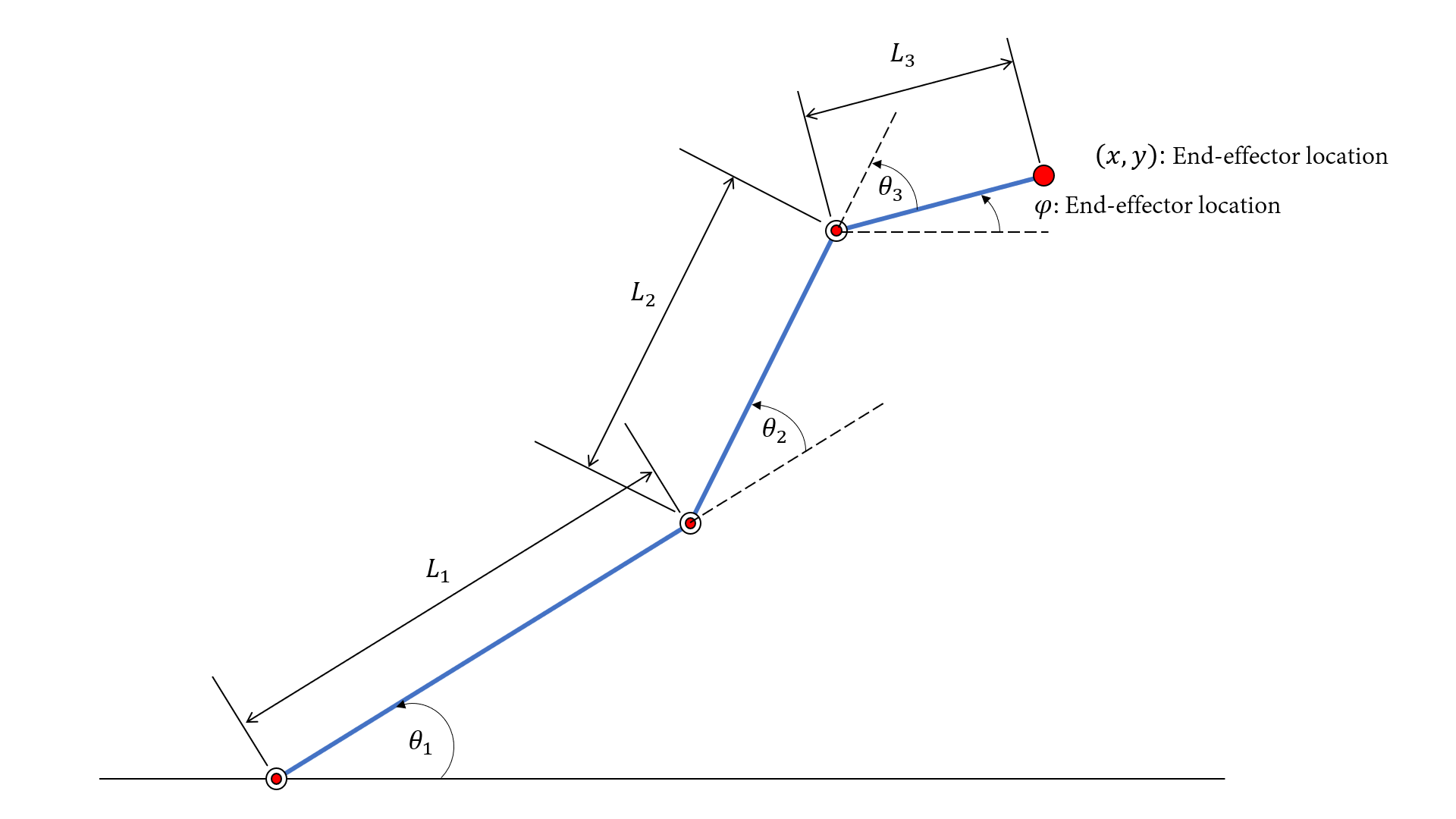
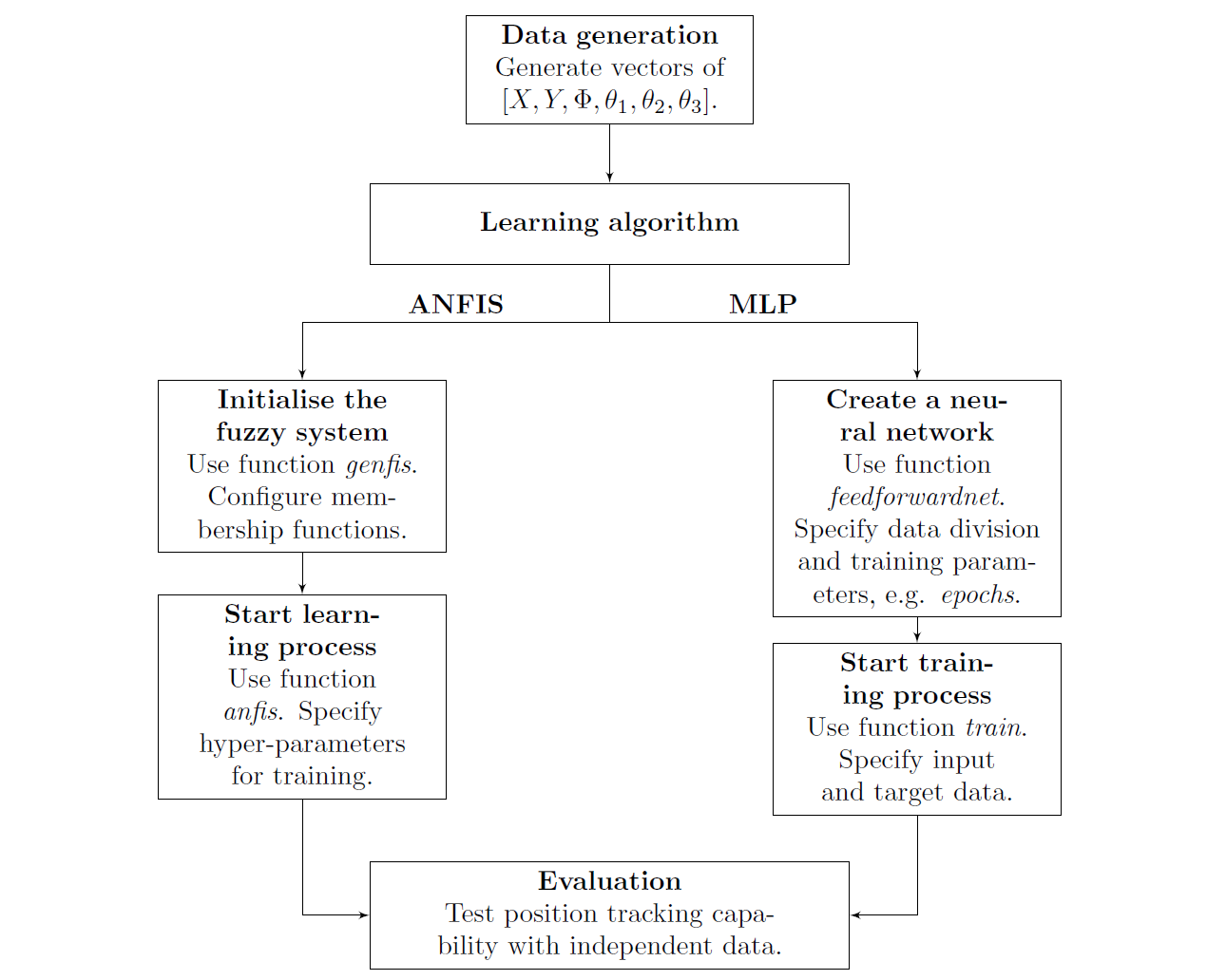
For the planar 3R arm shown in above figure, link lengths and the joint angles are specified with certain values or constraints. The inverse kinematics problem involves around the mapping from the Cartesian coordinates $X, Y$ to the joint angles $\theta_1,\theta_2,\theta_3$. Therefore, in order to train the models, data samples with certain mapping should be created beforehand. Finally, once the models are both learned from the dataset, evaluations will be taken to illustrate how well the models: Adaptive Neuro-Fuzzy Inference System (ANFIS) and Multiple Layer Perceptron (MLP) fit the training data. The overall process can be seen in the flowchart.
- LINK LENGTHS: $l_1=10$, $l_2=7$, $l_3=5$.
- ANGLE LIMITS: $\theta_i\in[0,\pi/2]$ for $i=1, 2, 3$.
Data generation
Since the geometrical configurations have been provided, this section firstly introduces how to creates the Cartesian localisation vectors through mapping: Forward Kinematics:
$$
\begin{equation}
X = l_1\times cos(\theta_1)+l_2\times cos(\theta_1+\theta_2)+l_3\times cos(\theta_1+\theta_2+\theta_3) \\
Y = l_1\times sin(\theta_1)+l_2\times sin(\theta_1+\theta_2)+l_3\times sin(\theta_1+\theta_2+\theta_3) \\
\Phi=\theta_1+\theta_2+\theta_3
\end{equation}
$$
Firstly, we generate three sets of angle values linearly varying from $0$ to $\pi/2$. Every angular vector should hold the same number of entries due to the subsequent vectorisation in forward kinematics equations. Then, the grid coordinates of three angles are produced to create the full combination of joint angles. Derived from the geometrics of the robot architecture, forward kinematics equations defined that each set of angular values are corresponding to a set of localisation values. Vectorisation is applied in the equations to generate $X,Y$ coordinates and the orientation $\Phi$ of the end-effector. Notably, all the six column vectors are in the same size.
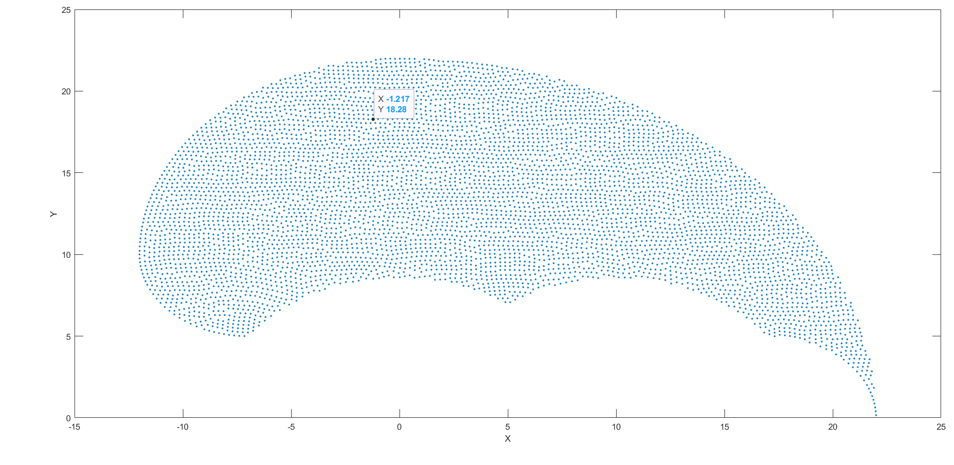
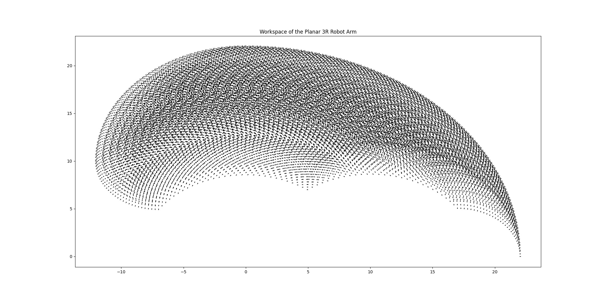
The six vectors: $\vec{X}, \vec{Y}, \vec{\Phi}, \vec{\theta_1},\vec{\theta_2},\vec{\theta_3}$ are concatenated elementwise to form a matrix in the shape of $[\text{Number of samples},6]$, which means the number of rows suggests the number of samples and the number of columns is the number of attributes of the kinematics. However, since the similar localisations $[x,y,\phi]$ correspond to similar angular configurations, a filter should be used to removed those replicates in Cartesian space. The filter can impose limit to the minimum distance within two Cartesian points to make the workspace slightly more sparse. The filtered workspace has a total number of 6179 points, illustrated below.
Implementations
Implementation of ANFIS
Dataset splits. A reasonable preprocessing step is to split the dataset into three parts: Train set, Validation set, and Test set. The recommended method is: K-Fold Cross Validation but that is a little bit complicated for this case (BUT I may try it later). I only apply one-time splitting, i.e. dividing the dataset into three parts with different percentages.
Off-the-shelf MATLAB function: dividerand. This is the function from Deep Learning Toolbox and it will generate three matrices containing randomised indices of train set, validation set and test set respectively.
Generate an FIS. Generate an Adaptive Neuro-Fuzzy Inference System (ANFIS). Before the initialisation, options including specifications of membership functions (MFs), important hyperparameters (like number of epochs) should be specified.
Off-the-shelf MATLAB function:
genfis: generates a single-output Sugeno fuzzy inference system (FIS) using a grid partition of the given input and output data.genfisOptions: creates a default option set for generating a fuzzy inference system structure usinggenfis.plotmf: plots the membership functions for an input or output variable in the fuzzy inference systemfis.
Training and validation. Learn the model from some epochs of training. Meanwhile, the model is fed with the validation set frequently to ensure a lowest validation error and to avoid overfitting.
Off-the-shelf MATLAB function:
anfis: tunes an FIS using the specified training data and options.anfisOptions: creates a default option set for tuning a Sugeno fuzzy inference system usinganfis.
Evaluation with independent test set. This is the final step for assessing how well the model does to fit the training data and show generalisation. Root Mean Squared Error (RMSE) can reveal the error in all three sets.
Off-the-shelf MATLAB function:
evalfis: evaluates the fuzzy inference systemfisfor the input values ininputand returns the resulting output values inoutput.evalfisOptions: creates an option set for theevalfisfunction with default options.plot: mainly for plotting errors in training process, MFs, data presentations, etc.
Self-defined codes to calculate RMSE: (Actually default options of anfis can make the training process output RMSE)
| |
Implementation of MLP
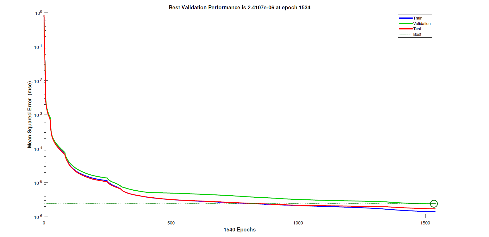
To implement Multi-Layer Perceptron (MLP), I use the same dataset but specify the division ratio in network configurations. feedforwardnet initialise a network and train tune the network based on given data. The original 6179-sample dataset is divided into the training set ($70%$), the validation set ($15%$) and the test set ($15%$). In terms of the architecture of the neural network, Duka (2014) had applied $[3,100,3]$ to solve IK problems but it required improvements due to its simple structure: only one hidden layer with 100 nodes. Therefore, the choice of $[12,12,6]$ has been made. The network has 12 neurons in both the first and the second hidden layer, and 6 neurons in the last hidden layer. Besides, there are 3 neurons in both input and output layers because three Cartesian space values are input to the model to predict three angles. Finally, the number of epochs is set at 4000, a higher value to where the network in fact terminates due to validation checks. Figure below demonstrates that less than 4000 epochs have been implemented to learn the training patterns.
*PyTorch Implementation of Neural Network
[26/04/2020] I implemented the NN model for IK problem of the planar 3R robot manipulator. The network architecture, input data and the output data are all the same as those in MATLAB implementations. However, there is no filter to sparse the workspace and there is no validation step in training. For optimiser,
Adamis used at the learning rate at 0.01.Adamoptimiser can yield quick convergence in loss function. But the results show that the positional errors are about 10 times larger than those of the MATLAB MLP model. I may attribute the reasons to theregion of computation. In the evaluations of MATLAB implementations, the models are evaluated on some local trajectories with fixed end-effector orientation. In these trajectories, the end-effector can access the points with the fixed pose at ease. However, in PyTorch implementation, all samples in the dataset are fed to the network and the network output predicted joint values on the whole workspace. It is known that many of the points in the workspace can be reached with various configurations of joint values. Those points are often leading to high positional errors. Another reason may be attributed to no sparse filter, which can definitely suppress multiple solutions. 🖇Code.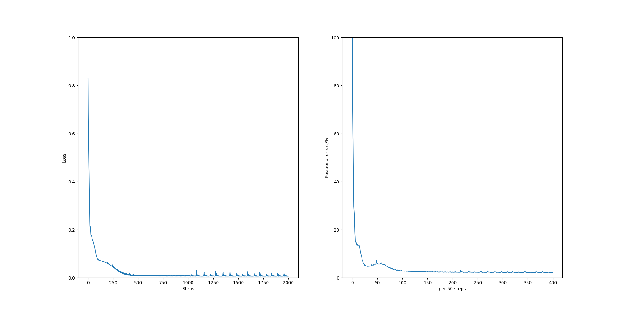
Evaluation
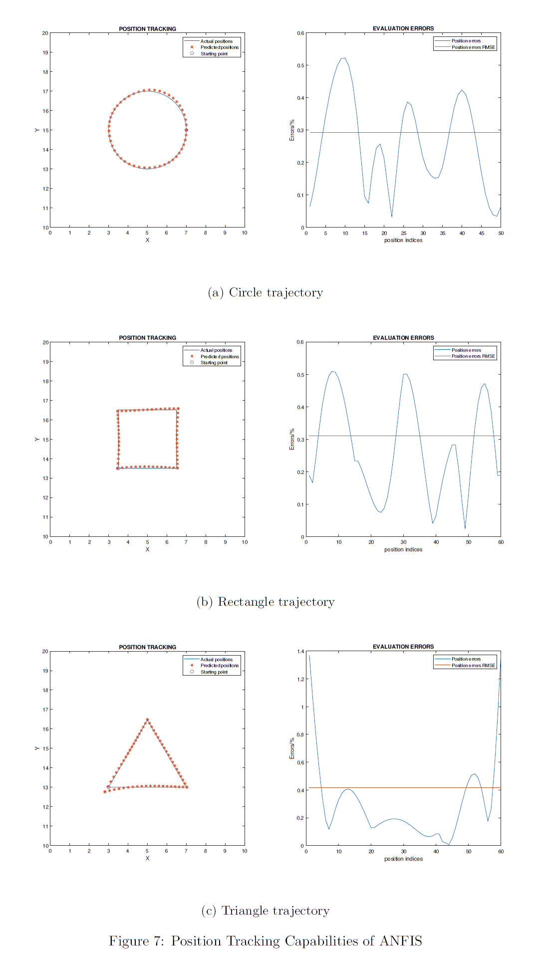
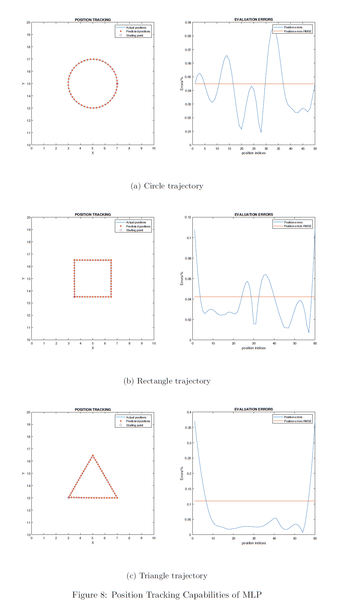
Evaluation of two types of models are implemented with independent data. Firstly, ground truth Cartesian coordinates $X,Y$ are generated from a part of the workspace. To study how the models fit the data in different scenarios, this report shows how three shapes are created and they are regarded as the hypothetical trajectories that the end-effector of the arm should track. The first shape is a circle whose centre is at $(5,15)$ and the radius is 2. The second shape is a square whose centre is also located at $(5,15)$ with a side length at 3. The last shape is an equilateral triangle with the same centre as the previous ones and the side length is 4. For all three trajectories, constant orientation of the end-effector is held at $3/4\pi$.
The vectors of $X$, $Y$ and $\Phi$ are input to the models to produce the corresponding angles $\theta_1$, $\theta_2$ and $\theta_3$ as the predicted values. Then forward kinematics are applied to the predictions of joint angles to produce the predicted Cartesian coordinates, noted as $X_{pred}$ and $Y_{pred}$. The approach to define how accurate the models fit the training data and how well the end-effector tracks the trajectories is to calculate the distances between the ground truth values $X$, $Y$ and the predictions $X_{pred}$, $Y_{pred}$. The way of doing this in the report is to derive the errors as the percentages of the total reach limit, $l_1+l_2+l_3$. Also, the Root Mean Squared Error (RMSE) is reported to show a overall performance in tracking the specific trajectory.
The results of the evaluation on ANFIS networks are shown in the first figure below. And the results of the evaluation on MLP networks are shown in following one.
Analysis of Results
According to figures above, it is obvious that MLP outperforms ANFIS in all experiments on three trajectories, given enough data (6179 samples). Generally, MLP yields in errors 10% as large as those of the ANFIS networks in both circle and rectangle trajectory tracking. Though the errors of the trained MLP network results in approximately 75% improvements from 0.4% to 0.1% in localisation errors while tracking the triangular trajectory. Another feature of triangular trajectory tracking is that the localisation errors are always larger than those of other shapes. ANFIS network achieved 0.4% RMSE of localisation errors, slightly larger than those of circular and rectangular trajectories. This slight difference is not shown in the results of the MLP network. The MLP model achieved the 0.4% RMSE in triangle shape but the RMSE in two other shapes' experiments have both dropped from 0.3% to about 0.04%.
Notably, all these large localisation errors in triangular trajectory tracking come from the left-bottom corner $(3,13)$ of the triangle. Recall that the orientation is specified at $3/4\pi$ and that means the end-effector of the robot arm reach all points on the trajectory with the same pose. However, since ground truth samples may involve around different small ranges of orientation values in different areas, the left-bottom corner corresponds to larger difference between the ground truth poses and the predicted poses. While around other two corners of the triangle, the orientations may differ but in a slight manner.
Conclusion
This post introduced two solutions to the problem of the inverse kinematics of a Planar 3R Manipulator: Adaptive Neuro-Fuzzy Inference System (ANFIS) and Multi-Layer Perceptron (MLP). The ANFIS solutions are small but effective models, with 24 rules for each and can be tuned within a total duration of three minutes. The localisation errors achieved by the ANFIS models are below a small level at 0.5% for experiments on tracking three trajectories. Also, an MLP model which has three hidden layers was trained for over 1500 epochs on the same dataset. Results demonstrate that the MLP network outperforms the ANFIS network in the current case. All Root Mean Square Errors (RMSE) of localisation distances are below 0.1% in position tracking. MATLAB codes of the implementation of the ANFIS and MLP networks are well commented and formatted, which can be seen in the Appendix.
References
See my report in GItHub repo: JinhangZhu/ias-coursework